Natural Selection and Loss Functions
Table Of Contents
Natural Selection is what allows our species (and images!) to improve over time. In this article we’ll implement a scoring mechanism, through which “Mona Lisa” will actually look like one.
Natural Selection
Natural selection is the process though which species adapt to their environments. If the evolution is a wheel, then natural selection is the force that spins it. Organism that are better adapted tend to produce more offspring and pass on their genes. This process favours genes that aided their bearers to survive/reproduce, increasing their number in the following generations.
In biology “fitness” is defined by how successful an organism is at reproduction.
Wikipedia says:
If an organism lives half as long as others of its species, but has twice as many offspring surviving to adulthood, its genes become more common in the adult population of the next generation.
… and also …
It is also equal to the average contribution to the gene pool of the next generation, made by the same individuals of the specified genotype or phenotype.
We, however, will define “fitness” as a difference between an organism and the ideal. Which is a bit vague, as there’s no obvious way of substituting one image from another and produce an integer. We’ll get back to that in a bit.
Loss functions
Genetic Algorithms (and Evolutionary Algorithms) are optimization algorithms that need a “goodness” of an organism, in order to decide whether to discard it. We’re going to implement two scoring methods, both based on loss functions. L1 Loss Function and L2 Loss Function are defined as follows:
$$ L1 = \sum_{i=0}^n \vert y_{true_i} - y_{predicted_i} \vert \newline L2 = \sum_{i=0}^n \left( y_{true_i} - y_{predicted_i} \right)^2 $$
n represents the size of the ideal image in pixels; we know, that both images have the exact same size, so it will
never out-of-range.
Both of these functions are used to covert an “object” or an “event”, to a real number representing its score. Which one should be picked then? In general L2 Loss Function is preferred in most of the cases. However, when the dataset has outliers, then L2 Loss Function does not perform well – it leads to much larger errors.
Cool, we have a way of calculating differences between images’ pixels. But how to calculate a difference between two pixels? That question was already answered in Art From Chaos. We take each of the pixels color channels and calculate their differences.
$$ f(O, S) = \sum_{i=0}^n \vert (r_2 - r_1)^2 + (g_2 - g_1)^2 + (b_2 - b_1)^2 \vert $$
Scoring mechanism
First, let’s define a trait whereby the rest of the system will be able to interact with scoring methods.
1pub trait FitnessFunction {
2    /// This method calculates the fitness of `second_image` relative to `first_image`.
3    ///
4    /// In other words, it returns a value describing difference between those two images. The higher the value, the
5    /// more those images are different from each other.
6    fn calculate_fitness(&self, first_image: &Image, second_image: &Image) -> usize;
7}
The method assumes that the first_image is the one being scored and second_image is the ideal. However, what’s nice
about these loss functions, is that they return absolute values – it does not matter which parameter is the ideal.
1// True for both L1 and L2
2assert_eq!(
3    scorer.calculate_fitness(first_image, second_image),
4    scorer.calculate_fitness(second_image, first_image)
5);
Implementation of L1: AbsoluteDistance
The implementation isn’t complex - first we fold each pixel pair to a usize, and then we sum those parts together to
produce the score. Actually, we can do both by using Iterator’s fold method.
 1fn fold_pixels(mut sum: usize, (p1, p2): (&Pixel, &Pixel)) -> usize {
 2    let diff_r = isize::from(p1.get_r()) - isize::from(p2.get_r());
 3    let diff_g = isize::from(p1.get_g()) - isize::from(p2.get_g());
 4    let diff_b = isize::from(p1.get_b()) - isize::from(p2.get_b());
 5
 6    sum += diff_r.unsigned_abs();
 7    sum += diff_g.unsigned_abs();
 8    sum += diff_b.unsigned_abs();
 9
10    sum
11}
12
13#[derive(Debug, Default)]
14pub struct AbsoluteDistance;
15
16impl FitnessFunction for AbsoluteDistance {
17    fn calculate_fitness(
18        &self,
19        first_image: &crate::models::Image,
20        second_image: &crate::models::Image,
21    ) -> usize {
22        first_image
23            .pixels()
24            .iter()
25            .zip(second_image.pixels().iter())
26            .fold(0usize, fold_pixels)
27    }
28}
Implementation of L2: SquareDistance
Implementation of SquareDistance is almost identical. The only difference is the squaring of color channels.
 1fn fold_pixels(mut sum: usize, (p1, p2): (&Pixel, &Pixel)) -> usize {
 2    let diff_r = isize::from(p1.get_r()) - isize::from(p2.get_r());
 3    let diff_g = isize::from(p1.get_g()) - isize::from(p2.get_g());
 4    let diff_b = isize::from(p1.get_b()) - isize::from(p2.get_b());
 5
 6    sum += diff_r.pow(2) as usize;
 7    sum += diff_g.pow(2) as usize;
 8    sum += diff_b.pow(2) as usize;
 9
10    sum
11}
12
13#[derive(Debug, Default)]
14pub struct SquareDistance;
15
16impl FitnessFunction for SquareDistance {
17    fn calculate_fitness(
18        &self,
19        first_image: &crate::models::Image,
20        second_image: &crate::models::Image,
21    ) -> usize {
22        first_image
23            .pixels()
24            .iter()
25            .zip(second_image.pixels().iter())
26            .fold(0usize, fold_pixels)
27    }
28}
Fixing “Mona Lisa”
Let’s wire up the scoring component with generation’s flow. During each generation, every specimens will be scored relatively to the ideal image. Using the scores we will select the best 51 organisms and discard the rest.
Since there’s no crossover functionality yet, we need to fill the emptied generation space somehow. Simplest solution: once we have 5 best specimens, we’ll copy them over multiple times, to get a new generation 100 strong.
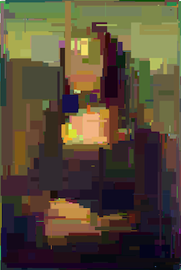
Mona Lisa (generation #10 000)
🤌
The image does look recognizable. And it’s still missing the last part – crossing. However, as it’s not “required”, the algorithm works and it produces acceptable results.
Next, we’ll implement the crossing function and we’ll see how much it improves algorithm’s efficiency – defined as the derivative of specimen score with respect to generation number.
Photo by Fernando Venzano on Unsplash
Why 5? No particular reason. There should be enough specimen to fill the generation space again by combining them in varied ways. It could be more than 5, but we need to remember, that the goal of dropping those “bad” images is to discard mutations that resulted in decreasing overall “goodness”. ↩︎
Interested in my work?
Consider subscribing to the RSS Feed or joining my mailing list: madebyme-notifications on Google Groups .
Disclaimer: Only group owner (i.e. me) can view e-mail addresses of group members. I will not share your e-mail with any third-parties — it will be used exclusively to notify you about new blog posts.